Binius STARK Proof Systems Over Binary Field
1. Multilinear Polynomial $P(x_1,…,x_n)$
A univariate polynomial (i.e., a polynomial $P(x)$ with only one variable) can express the execution trace of a program. The “trace” refers to the sequence of states or outputs generated during the execution of a program. Each state in the sequence corresponds to a specific step in the program’s execution, and these states can be encoded as values of the univariate polynomial.
Mapping the program’s execution trace to a univariate polynomial involves associating each step of the program with a unique input value, typically represented by integers or elements from a finite field. The outputs or states generated by the program at each step are used as the corresponding coefficients of the polynomial. The resulting polynomial encapsulates the entire execution trace, allowing for the verification of computational integrity without revealing the actual states or inputs.
The advantage of using univariate polynomials to represent program execution traces lies in the ease of applying algebraic methods for verification and analysis. For example, properties of the program, such as completeness and soundness, can be represented and verified by examining the divisibility of the corresponding polynomial. While univariate polynomials are effective for representing simple programs or sequences of states, multilinear polynomials extend this concept to more complex scenarios. A multilinear polynomial is a polynomial that contains two or more variables, with each variable representing different aspects of the program’s execution.
Multilinear polynomials can be computed extremely efficiently over binary fields, which offers significant advantages in CPU-based computing environments. Binary fields (also known as finite fields of characteristic 2) are well-suited for representing and processing data in binary form, which is the native format for computing systems. Operations on binary polynomials, such as addition, multiplication, and evaluation, can be performed efficiently using algorithms optimized for binary arithmetic.
In practical applications, the use of multilinear polynomials over binary fields can enhance the performance and scalability of program analysis and verification techniques. Multilinear polynomials can be used to represent and verify complex protocols and construct zero-knowledge proofs. By leveraging the mathematical properties of polynomials and the efficiency of binary computation, this method allows for rigorous examination of program behavior, even in complex and high-dimensional environments.
2. Efficient Binary and Binary Finite Fields
Binary computation is at the core of modern computing systems. In binary representation, data is encoded using 0 and 1, corresponding to the off and on states in a digital circuit. The binary system is fundamental because it perfectly aligns with the physical properties of electronic devices, which operate with only two distinct states.
Advantages of Binary Computation:
- Simplicity and Robustness: Binary computation is inherently simple since it only uses two states, which reduces the likelihood of errors caused by noise or signal degradation. This robustness makes it ideal for data computation and processing.
- Compatibility with Logic Gates: Binary data can be easily manipulated using logic gates such as AND, OR, and XOR, which are the building blocks of digital circuits. These gates perform operations directly on binary inputs, making the design and implementation of digital systems straightforward and efficient.
- Efficient Arithmetic Operations: Arithmetic operations in binary, such as addition, subtraction, multiplication, and division, can be efficiently implemented using algorithms designed for binary arithmetic. For instance, binary addition can be performed using simple bitwise operations with carry propagation, and multiplication can be executed using shift-and-add techniques.
- Scalability: Binary systems scale well as data sizes increase. Modern processors are optimized to handle binary data in standard sizes, such as 16-bit, 32-bit, and 64-bit, enabling efficient processing of large datasets.
A binary finite field, typically denoted as $ GF(2^m) $, is a finite field with $ 2^m $ elements, where each element is represented by an $ m $-bit binary string. These finite fields play a crucial role in several areas of computer science, particularly in coding theory, cryptography, and error correction.
Structure and Properties:
- Field Elements: In the binary finite field $GF(2^m)$, elements can be expressed as polynomials with coefficients from $ \{0,1\} $. The addition and multiplication of these elements are defined through polynomial arithmetic modulo an irreducible polynomial of degree $ m $.
- Field Arithmetic: Arithmetic operations in binary finite fields, such as addition, subtraction, multiplication, and division, are defined in a way that ensures the properties of the field. Addition and subtraction are performed using bitwise XOR operations, while multiplication involves polynomial multiplication followed by modular reduction. Division is usually implemented by computing multiplicative inverses using the extended Euclidean algorithm.
- Efficiency: Binary finite fields are highly efficient for computation because their arithmetic operations can be performed using simple bitwise operations and shifts. This efficiency is especially important in hardware implementations, where operations must be carried out quickly and with minimal power consumption.
Applications of Binary Finite Fields:
- Cryptography: Binary finite fields form the foundation of cryptographic algorithms, such as elliptic curve cryptography (ECC). ECC relies on the algebraic structure of elliptic curves over finite fields and provides strong security with relatively small key sizes, making it suitable for use in resource-constrained environments.
- Error-Correcting Codes: Binary finite fields are used to construct error-correcting codes, such as Reed-Solomon codes and BCH codes, which are essential for ensuring data integrity in communications and storage. These codes leverage the arithmetic properties of finite fields to detect and correct errors in transmitted or stored data, enhancing the reliability of digital systems.
- Polynomial Representation and Fast Algorithms: Binary finite fields enable efficient implementation of algorithms that rely on polynomial representation. Fast algorithms for polynomial multiplication, such as the Karatsuba algorithm, can be applied within the context of binary finite fields, achieving high-speed computation in specific applications.
3. Preliminaries
The smallest possible field is the arithmetic field modulo 2, with the following addition and multiplication tables.
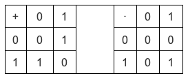
By extending this, we can create larger binary fields: starting from $F_2$ (integers modulo 2), and then defining $x² = x + 1$, we obtain the following addition and multiplication tables.

By repeating this construction, binary fields can be extended to arbitrary sizes. The elements are defined as follows:
- $x_0$ satisfies $x_0²=x_0 + 1$;
- $x_1$ satisfies $x_1²=x_1 ∙ x_0+1$;
- $x_2$ satisfies $x_2²=x_2 ∙ x_1+1$;
- $x_3$ satisfies $x_3²=x_3 ∙ x_2+1$.
This is known as a tower construction with Multilinear Lagrange Base, where each consecutive extension can be viewed as adding a new layer to the tower. This has the advantage that embedding one extension into the others is achieved trivially by padding zero coefficients. The construction proceeds inductively:
- Start from $τ_0=F_2$
- Set $τ_1=F_2[x_0]/(x_0²+x_0+1)$
- Continue $τ_k=F_2[x_1^k]/(x_{k−1}²+x_{k−1}*x_{k-2}+1)$
These numbers can be represented as bit lists, such as $1100101010001111$. The first bit represents a multiple of $1$, the second bit represents $x_0$, and the subsequent bits represent the following multiples: $x_1$, $x_1 \cdot x_0$, $x_2$, $x_2 \cdot x_0$, etc.
These encodings have the following decomposition properties:
\[
1100101010001111
=11001010+10001111∙x_3
=1100+1010∙x_2+1000∙x_3+1111∙x_2x_3
=11+10∙x_2+10∙x_2x_1+10∙x_3+11∙x_2x_3+11∙x_1x_2x_3
=1+x_0+x_2+x_2∙x_1+x_3+x_2∙x_3+x_0∙x_2x_3+x_1∙x_2∙x_3+x_0∙x_1∙x_2∙x_3
\]
Represent the binary field elements as integers, using bit representation, with the most significant bits on the right.
For example:
- $ 1 = 1 $,
- $ x_0 = 01 = 2 $,
- $ 1 + x_0 = 11 = 3 $,
- $ 1 + x_0 + x_2 = 11001000 = 19 $, etc.
Thus, in this representation, $1100101010001111$ equals $61779$.
Addition in Binary Fields: Addition is performed via XOR. This means $x + x = 0$ for any $x$. Subtraction is done by negating and then applying XOR.
Multiplication in Binary Fields: To multiply two elements $x \cdot y$, first split each number into two halves:
\[ x = L_x + R_x \cdot x_k $ and $ y = L_y + R_y + x_k \]
Then, break down the multiplication:
\[
x \cdot y = (L_x \cdot L_y) + (L_x \cdot R_y) \cdot x_k + (R_x \cdot L_y) \cdot x_k + (R_x \cdot R_y) \cdot x_k²,
\]
where $x_k² = x_{k-1} \cdot x_k + 1$.
Division in Binary Fields: Combine multiplication with inversion. For example, $\frac{3}{5}$. First, compute the inverse $\frac{1}{5} = 5^{14} = 14$, and then perform the multiplication $3 \cdot 14 = 9$.
Addition and multiplication tables for four-bit binary field elements are as follows:
4. Binius Stark Scheme
> Note: All multiplication and addition are based on the binary field operations described earlier in tables 3 and 4.
The following system framework is from Binius. Appropriate modifications have been made for ease of explanation.
Step 1 (Flatten): In the Flatten phase, encode the hypercube into a matrix 1
\[
\begin{bmatrix}
0 & 0 & 1 & 1 \\
1 & 0 & 0 & 1 \\
1 & 1 & 0 & 1 \\
1 & 1 & 1 & 1
\end{bmatrix}
\]
Step 2 (RS Extension): The values in matrix 1 are treated as the values of a polynomial, with the corresponding x-coordinates $r = \{0, 1, 2, 3\}$. At $r = \{4, 5, 6, 7\}$, apply the Reed-Solomon (RS) extension to matrix 1 to obtain the next matrix 2
\[
\begin{bmatrix}
1 & 0 & 0 & 1 \\
0 & 0 & 1 & 1 \\
1 & 0 & 0 & 0 \\
1 & 1 & 1 & 1
\end{bmatrix}
\]
Example: The first row of matrix 1 (0,0,1,1) is viewed as the binary representation (0,0) and (1,1) with a bit width of 2, which gives the polynomial values 0 and 3. The corresponding x-coordinates are $r = 0$ and $r = 1$, from which a first-degree polynomial can be constructed. At $r = 2, 3$, compute the values of the polynomial (1 and 2). Decompose 1 and 2 into binary (1,0) and (0,1), yielding the first row of matrix 2 as (1,0,0,1).
Step 3 (Merkle Commitment): Construct a Merkle tree for matrix 1 and matrix 2, and the Merkle root (ROOT) serves as the commitment.
Step 4 (Goal): The prover provides the polynomial value $P(r_1, r_2, r_3, r_4)$ at a random point $r = (r_1, r_2, r_3, r_4)$. The verifier calculates the polynomial value at the same point from a different perspective to ensure that the prover’s value is correct, thus confirming that the provided polynomial is correct.
Prover: At some random point, such as $r = \{2, 0, 3, 4\}$, the prover calculates the polynomial value
\[
P(2, 0, 3, 4) = 14
\]
and sends 14 to the verifier.
Verifier: (1) Split $r = \{2, 0, 3, 4\}$ into two parts:
- Part 1: $ \{2, 0\} $ represents the linear combination for the columns.
- Part 2: $ \{3, 4\} $ represents the linear combination for the rows.
(2) Compute the “tensor product” for the columns and rows:
- Column tensor product: $ \otimes_{i=0}^{1}(1- r_i, r_i) $
- Row tensor product: $ \otimes_{i=2}^{3}(1 — r_i, r_i) $
This generates a list containing all possible products from each set.
(3) For the row part, the result of the tensor product is:
\[ [(1 — r_2) \cdot (1 — r_3), r_2 \cdot (1 — r_3), (1 — r_2) \cdot r_3, r_2 \cdot r_3] \]
Substituting $r_2 = 3$ and $r_3 = 4$ into $r = \{2, 0, 3, 4\}$, we get:
\[
[10, 15, 8, 12]
\]
(4) Perform a linear combination of the rows to compute a new “row” $t’$. Multiply each row by its corresponding coefficient:
\[
[0, 0, 1, 1] \cdot 10 + [1, 0, 0, 1] \cdot 15 + [1, 1, 0, 1] \cdot 8 + [1, 1, 1, 1] \cdot 12 = [11, 4, 6, 1]
\]
The coefficients come from the list computed earlier.
(5) Perform a linear combination of $[3, 2, 0, 0]$ with $[11, 4, 6, 1]$:
\[
3 \cdot 11 + 2 \cdot 4 + 0 \cdot 6 + 0 \cdot 1 = 14
\]
The result gives the value 14.
Step 5 (Goal): From two different perspectives, we obtain equal results.
- Method A: Perform an RS extension on matrix 1 to obtain matrix 2; then apply a row linear combination to the last two columns of matrix 2, followed by column decomposition to obtain matrix 4.
- Method B: Perform a row linear combination on the values of matrix 1, followed by column decomposition, and then perform an RS extension to obtain matrix 4.
Method A:
(1) The prover performs an RS extension on matrix 1 to obtain matrix 2
\[
\begin{bmatrix}
1 & 0 & 0 & 1 \\
0 & 0 & 1 & 1 \\
1 & 0 & 0 & 0 \\
1 & 1 & 1 & 1
\end{bmatrix}
\]
The prover sends the last two rows of matrix 2 to the verifier.
(2) The verifier performs a linear combination of the last two columns of matrix 2
\[
[0, 1] \cdot 10 + [1, 1] \cdot 15 + [0, 0] \cdot 8 + [1, 1] \cdot 12 = [3, 9]
\]
(3) The verifier decomposes $[3, 9]$ into binary, obtaining $[1, 1, 0, 0]$ and $[1, 0, 0, 1]$.
Method B:
(1) The prover performs a linear combination on matrix 1
\[
[0, 0, 1, 1] \cdot 10 + [1, 0, 0, 1] \cdot 15 + [1, 1, 0, 1] \cdot 8 + [1, 1, 1, 1] \cdot 12 = [11, 4, 6, 1]
\]
The prover sends $[11, 4, 6, 1]$ to the verifier.
(2) The verifier decomposes $[11, 4, 6, 1]$ into binary to obtain matrix 3
\[
\begin{bmatrix}
1 & 0 & 0 & 1 \\
1 & 0 & 1 & 0 \\
0 & 1 & 1 & 0 \\
1 & 0 & 0 & 0
\end{bmatrix}
\]
(3) Perform an RS extension on matrix 3 to obtain matrix 4
\[
\begin{bmatrix}
0 & 0 & 1 & 1 \\
1 & 0 & 1 & 0 \\
1 & 1 & 0 & 0 \\
1 & 1 & 0 & 1
\end{bmatrix}
\]
The last two columns of matrix 4 obtained from Method A and Method B are equal.
5. Conclusion
This article first introduced the addition, subtraction, multiplication, and division in binary fields. It then presented the core principles of the Binius STARK Proof Systems. Due to the linear relationships of multilinear polynomials, both the prover and the verifier, when calculating the polynomial values from different perspectives, obtain equal results. Furthermore, this linear relationship ensures that the order of performing RS extension and linear combination on the matrix does not affect the outcome.